2.6.4. TikZ Goodies
- Homepage
TikZ Goodies is a small and simple collection of TikZ packages for drawing:
- CTAN Package
- Documentation
- Documentation
Various kinds of timing diagrams (not hardware-oriented).
Attention
You may want to have a look at TikZ-Timing too if you want to draw some hardware-oriented timing diagrams.
tikzgoodies/timing-diagrams/basic.tex, in
Figure 2.22.
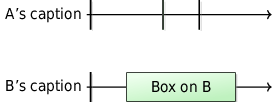
Figure 2.22 Basic Timing-Diagram example without additionals
tikzgoodies/timing-diagrams/timeline.tex, in
Figure 2.23.
![\begin{tikzpicture}
\draw (-1,1.5) node[rotate=90] (systemc) {\textsf{\large SystemC}};
\draw[dashed] (-1,0) -- (9,0);
\draw (-1,-2) node[rotate=90] (jtlm) {\textsf{\large jTLM}};
% SystemC
\tline{A}{2.1};
\tcaption{A}{A};
\tline{B}{1};
\tcaption{B}{B};
\ttimeline{A}{5};
\ttimeline{B}{5};
% jTLM
\tline{P}{-1.5};
\tcaption{P}{P};
\tline{Q}{-2.6};
\tcaption{Q}{Q};
\ttimeline{P}{5};
\ttimeline{Q}{5};
\ttick{A};
\ttextU{A}{f()};
\tskiptext{A}{2}{\texttt{\scriptsize wait(20)}};
\ttick{A};
\tskip{A}{1};
\ttick{A};
\ttick{B}
\tskip{B}{1};
\ttick{B};
\tskip{B}{1};
\ttick{B};
\tskip{B}{2};
\ttick{B};
\ttick{P}
\ttextU{P}{g()};
\tskiptext{P}{2}{\scriptsize awaitTime}
\ttick{P};
\tbox{P}{1.5}{h()};
% just so that the final picture looks pretty
\tbox{Q}{1.3}{i()};
\tskip{Q}{1};
\ttick{Q};
\tskip{Q}{.5};
\tbox{Q}{2}{j()};
\end{tikzpicture}
%Local variables:
% coding: utf-8
% mode: text
% mode: rst
% End:
% vim: fileencoding=utf-8 filetype=tex :](../../_images/tikz-0e841ca006d57952529a2fcc8699467bb00eedff.png)
Figure 2.23 Timeline-Diagram example with ticks and tasks
tikzgoodies/timing-diagrams/annotations.tex, in
Figure 2.24.
![\begin{tikzpicture}
\tline{real}{0};
\tline{model}{2};
\ttimeline{real}{8.5};
\ttimeline{model}{8.5};
\tcaption{real}{Real system};
\tcaption{model}{SystemC model};
\tskip{real}{.5};
\tskip{model}{.5};
\path (currentrealU) coordinate (endzooma);
\tbox{real}{7}{\texttt{compute()}};
\path (currentrealU) ++(-.04, 0) coordinate (endzoomb);
\tstrongtick{real};
\ttextarrowU{real}{\texttt{commit()}};
\tstrongtick{model};
\path (currentmodelL) ++(-.04, 0) coordinate(startzooma);
\path (currentmodelL) ++( .04, 0) coordinate(startzoomb);
\ttextarrowU{model}{\texttt{compute()}};
\tskip{model}{.04};
\tskiptext{model}{6.92}{\texttt{wait()}};
\tskip{model}{.04};
\tstrongtick{model};
\ttextarrowU{model}{\texttt{commit()}};
\path (startzoomb -| endzoomb) coordinate (topright);
\path (barycentric cs:startzoomb=.5,endzooma=.5) coordinate (tmpa);
\path (barycentric cs:topright=.5,endzoomb=.5) coordinate (tmpb);
\draw[very thin,color=black!70!white] (startzooma) -- (endzooma);
\draw[very thin,color=black!70!white] (startzoomb) .. controls (tmpa) and (tmpb) .. (endzoomb);
\end{tikzpicture}
%Local variables:
% coding: utf-8
% mode: text
% mode: rst
% End:
% vim: fileencoding=utf-8 filetype=tex :](../../_images/tikz-cb97e7fbb68f69ac90e3efc7b923497e09a87d88.png)
Figure 2.24 Timing-Diagram example with annotations
tikzgoodies/timing-diagrams/callouts.tex, in
Figure 2.25.
![\begin{tikzpicture}[scale=.8]
\def\one{\raisebox{-2pt}{\large\ding{192}{ }}}
\def\two{\raisebox{-1.5pt}{\large\ding{193}{ }}}
\def\three{\raisebox{-2pt}{\large\ding{194}{ }}}
\tikzstyle{arrow}=[->,line width=.05cm,draw=red!90!blue!60!black]
\tline{A}{3};
\tcaption{A}{A};
\tline{B}{2};
\tcaption{B}{B};
\tline{C}{1};
\tcaption{C}{C};
\tline{T}{-1.5}
\tcaption{T}{OS thread};
\ttimeline{A}{10};
\ttimeline{B}{10};
\ttimeline{C}{10};
\ttimeline{T}{10};
\tbox{B}{1}{};
\tcatchup{C}{B};
\tbox{C}{1}{};
\tcalloutU[(-.8,2.5)]{C}{\texttt{during(42, routine);}}
\tcatchup{B}{C};
\tcatchup{T}{C};
\draw[arrow] (currentCL) -- node[left] {
\begin{tabular}{r}
\one create\\thread
\end{tabular}
} (currentTU);
\tbox{T}{4}{\texttt{routine}};
\tskiptextL{C}{4}{\two \texttt{wait(42)}\vspace{-2em}};
\tbox{B}{1.5}{};
\tcatchup{A}{B};
\tbox{A}{1}{};
\tcatchup{B}{A};
\tbox{B}{1}{};
\draw[arrow] (currentTU) -- node[right] {
\begin{tabular}{l}
\three join\\thread
\end{tabular}
} (currentCL);
\tbox{C}{1}{};
\tcatchup{A}{C};
\tbox{A}{1}{};
\tcatchup{B}{A};
\tbox{B}{1}{};
\end{tikzpicture}
%Local variables:
% coding: utf-8
% mode: text
% mode: rst
% End:
% vim: fileencoding=utf-8 filetype=tex :](../../_images/tikz-571cb7e681f21407d8b54b173ad5b9f524080975.png)
Figure 2.25 Timing-Diagram example with callouts (synchronizations)
Arrows (compact)
tikzgoodies/timing-diagrams/arrows-compact.tex, in
Figure 2.26.
![\begin{tikzpicture}[scale=.7]
\tline{sc}{2};
\tcaption{sc}{SystemC};
\tline{ace}{0};
\draw (currentace) ++ (9,-.3) node {Simulated time};
\tcaption{ace}{P/T Solver};
\ttimeline{sc}{10};
\ttimeline{ace}{10};
\tremember{sc}{before};
\tlonglighttick{sc};
\tskip{sc}{1.5};
\tlonglighttick{sc};
\tskip{sc}{1.5};
\tlonglighttick{sc};
\tskip{sc}{2};
\trecall{sc}{before};
\tbox{sc}{6}{Functional (1)};
\ttextarrowU{sc}{
\begin{tabular}{c}
SystemC reads\\temperature
\end{tabular}
};
\tarrowUL{sc}{ace}{};
\draw (tmpmid) node[fill=white,inner sep=1pt] {(2)};
\tremember{ace}{before};
\tlonglighttick{ace};
\tskip{ace}{1.5};
\tlonglighttick{ace};
\tskip{ace}{1.5};
\tlonglighttick{ace};
\tskip{ace}{2};
\trecall{ace}{before};
\tbox{ace}{6}{Non-functional (3)};
\tarrowLU{ace}{sc}{};
\draw (tmpmid) node[anchor=west] {(4)};
\tbox{sc}{2}{...};
\end{tikzpicture}
%Local variables:
% coding: utf-8
% mode: text
% mode: rst
% End:
% vim: fileencoding=utf-8 filetype=tex :](../../_images/tikz-9b8a67386e54694fe22adda091e9151fbac0a1ad.png)
Figure 2.26 Timing-Diagram example with arrows (compact)
Arrows (stretched)
tikzgoodies/timing-diagrams/arrows-stretched.tex, in
Figure 2.27.
![\begin{tikzpicture}[scale=.7]
\tline{sc}{2};
\tcaption{sc}{SystemC};
\tline{ace}{0};
\tcaption{ace}{P/T Solver};
\draw (currentace) ++ (9,-.3) node {Simulated time};
\ttimeline{sc}{10};
\ttimeline{ace}{10};
\tbox{sc}{1}{(1)};
\ttextarrowU{sc}{end of instant $t_{i}$};
\tcatchup{ace}{sc};
\coordinate (sceoi) at (currentscL);
\tskip{sc}{6};
\ttick{sc};
\ttextarrowU{sc}{next instant $t_{i+1}$};
\tarrowCoord{(sceoi)}{(currentaceU)}{};
\draw (tmpmid) node[anchor=east] {(2)};
\tbox{ace}{6}{non-functional simu (3)};
% \tcalloutL{ace}{No IT};
\ttick{sc};
\tarrowLU{ace}{sc}{};
\draw (tmpmid) node[anchor=west] {(4)};
% \tcalloutU{sc}{Continue};
\tbox{sc}{1}{...};
\end{tikzpicture}
%Local variables:
% coding: utf-8
% mode: text
% mode: rst
% End:
% vim: fileencoding=utf-8 filetype=tex :](../../_images/tikz-fbf34fdbecc4fab4b7d69d03dee0bf3701419a36.png)
Figure 2.27 Timing-Diagram example with arrows (stretched)
tikzgoodies/timing-diagrams/events.tex, in
Figure 2.28.
![\begin{tikzpicture}
\tikzstyle{arrow}=[->,line width=.05cm,draw=red!90!blue!60!black]
\tline{S}{6};
\tline{M}{5};
\tline{E}{2};
\tline{T}{0}
\tline{F}{-2};
\tline{Eb}{-5};
\tline{Tb}{-7}
\coordinate (n1) at (-2.5,-.5);
\coordinate (n2) at (-2.5,4);
\draw [decoration={brace,amplitude=10pt},decorate] (n1) to (n2);
\coordinate (o1) at (-2.5,-7.5);
\coordinate (o2) at (-2.5,-1.5);
\draw [decoration={brace,amplitude=10pt},decorate] (o1) to (o2);
\draw (barycentric cs:n1=.5,n2=.5) ++(-10pt,0) node[anchor=south,rotate=90] {\large\textsf{(a) Naive Temperature Model}};
\draw (barycentric cs:o1=.5,o2=.5) ++(-10pt,0) node[anchor=south,rotate=90] {\large\textsf{(b) Proposed Approach}};
\tcaption{S}{Real System};
\ttimeline{S}{8};
\tskip{S}{.3};
\tstartbrace{S};
\tevent{S}; \tskip{S}{1.5};
\tevent{S}; \tskip{S}{1.3};
\tevent{S}; \tskip{S}{1.2};
\tendbrace{S}{\texttt{f(); wait(40);}};
\tstartbrace{S};
\tskip{S}{.2};
\tevent{S}; \tskip{S}{.8};
\tevent{S}; \tskip{S}{.7};
\tevent{S}; \tskip{S}{.5};
\tevent{S}; \tskip{S}{.5};
\tevent{S}; \tskip{S}{.8};
\tevent{S};
\tendbrace{S}{\texttt{g(); wait(35);}};
\tcaption{M}{
\begin{tabular}{r}
Loosely-Timed\\Model
\end{tabular}
};
\ttimeline{M}{8};
\tskip{M}{.3};
\foreach \x in {10,0,-10} {
\teventA{M}{\x};
}
\tskip{M}{4};
\foreach \x in {25,15,5,-5,-15,-25} {
\teventA{M}{\x};
}
\tskip{M}{2.5};
\tcaption{E}{Energy};
\ttimeline{E}{8};
\draw[red!50!black,thick] (currentE) ++(0,.3) -- ++(.3,0) --
node[right] {+3} ++(0,.6) -- ++(4,0) --
node[right] {+6} ++(0,1.2) -- node[near end,below]{total=9} ++(3.5,0)
;
\tcaption{T}{Temperature};
\ttimeline{T}{8};
\draw[blue!50!black,thick] (currentT) ++(0,.3) -- ++(.3,0) --
coordinate[at end](peak1) ++(0,.6) .. controls +(1,-.2) .. ++(4,-.3) --
coordinate[at end](peak2) ++(0,1) .. controls +(1,-.5) .. ++(3.5,-.8)
;
\draw (peak1) node[draw,circle,thick](peak1){};
\draw (peak2) node[draw,circle,thick](peak2){};
\draw (barycentric cs:peak1=.5,peak2=.5) ++(0,.1) node[inner sep=0](peaks){
\begin{tabular}{c}
Unrealistic\\peaks
\end{tabular}
};
\draw [arrow] (peaks) -- (peak1);
\draw [arrow] (peaks) -- (peak2);
\tcaption{F}{Frequency};
\ttimeline{F}{8};
\tskip{F}{.3};
\tbox{F}{4}{$\frac{3}{40}$ trans/sec};
\tbox{F}{3.5}{$\frac{6}{35}$ trans/sec};
\tcaption{Eb}{Energy};
\ttimeline{Eb}{8};
\draw[red!50!black,thick] (currentEb) ++(0,.3) -- ++(.3,0) --
++(4,.6)
-- node[at end,right]{total=9} ++(3.5,1.2)
;
\tcaption{Tb}{Temperature};
\ttimeline{Tb}{8};
\draw[blue!50!black,thick] (currentTb) ++(0,.3) -- coordinate[at end](start)++(.3,0);
\path (start)
++(4,.6) coordinate (x1)
++(3.5,.3) coordinate(x2);
\draw[blue!50!black,thick,bend left=5] (start) to (x1);
\draw[blue!50!black,thick,bend left=5] (x1) to (x2);
;
\end{tikzpicture}
%Local variables:
% coding: utf-8
% mode: text
% mode: rst
% End:
% vim: fileencoding=utf-8 filetype=tex :](../../_images/tikz-696ea4ad5514908d0d17157367698f16df2e440f.png)
Figure 2.28 Timing-Diagram example with events as vertical arrows
- CTAN Package
- Documentation
- Documentation
Specific kind of execution stacks (typically to illustrate assembly language notions).
Minimal
tikzgoodies/drawstack/minimal.tex, in
Figure 2.29.
![% In context of the Sphinx TikZ extension we can not use the specific
% drawstack environment here and have to encapsulate it into a standard
% tikzpicture environment --> write the full declaration with \stacktop{}
% at the beginning and \stackbottom{} on the end.
\begin{tikzpicture}[x=0.7cm,y=0.7cm]
\stacktop{} % do not remove
%% now we on \begin{drawstack}
%% %%%%%%%%%%%%%%%%%%%%%%%%%%%%%%%%%%%%%%%%%%%%%%%%%%%%%%%%%%%%%%%%%%%%%%%%%%
\small
% Within the environment, draw stack elements with \cell{...}
\cell{First cell}
\cell{Second cell}
%% %%%%%%%%%%%%%%%%%%%%%%%%%%%%%%%%%%%%%%%%%%%%%%%%%%%%%%%%%%%%%%%%%%%%%%%%%%
%% now we into \end{drawstack}
\stackbottom{} % do not remove
\end{tikzpicture}
%Local variables:
% coding: utf-8
% mode: text
% mode: rst
% End:
% vim: fileencoding=utf-8 filetype=tex :](../../_images/tikz-8d339dca608cd31ff224d5ac03a270ac44123fa2.png)
Figure 2.29 Minimalistic execution stack example
Frames
tikzgoodies/drawstack/frames.tex, in
Figure 2.30.
![% In context of the Sphinx TikZ extension we can not use the specific
% drawstack environment here and have to encapsulate it into a standard
% tikzpicture environment --> write the full declaration with \stacktop{}
% at the beginning and \stackbottom{} on the end.
\begin{tikzpicture}[x=0.7cm,y=0.7cm]
\stacktop{} % do not remove
%% now we on \begin{drawstack}
%% %%%%%%%%%%%%%%%%%%%%%%%%%%%%%%%%%%%%%%%%%%%%%%%%%%%%%%%%%%%%%%%%%%%%%%%%%%
\small
\startframe
\cell{First cell}
\cell{Second cell}
\finishframe{Some stack frame}
\cell{Not interesting}
\startframe
\cell{\scriptsize Next stack frame}
\cell{\scriptsize Next stack frame}
\finishframe{Another stack frame}
%% %%%%%%%%%%%%%%%%%%%%%%%%%%%%%%%%%%%%%%%%%%%%%%%%%%%%%%%%%%%%%%%%%%%%%%%%%%
%% now we into \end{drawstack}
\stackbottom{} % do not remove
\end{tikzpicture}
%Local variables:
% coding: utf-8
% mode: text
% mode: rst
% End:
% vim: fileencoding=utf-8 filetype=tex :](../../_images/tikz-c90e0d29a3727280a9badca2de96db298815454d.png)
Figure 2.30 Execution stack example with grouped cells in frames
Padding
tikzgoodies/drawstack/padding.tex, in
Figure 2.31.
![% In context of the Sphinx TikZ extension we can not use the specific
% drawstack environment here and have to encapsulate it into a standard
% tikzpicture environment --> write the full declaration with \stacktop{}
% at the beginning and \stackbottom{} on the end.
\begin{tikzpicture}[x=0.7cm,y=0.7cm]
\stacktop{} % do not remove
%% now we on \begin{drawstack}
%% %%%%%%%%%%%%%%%%%%%%%%%%%%%%%%%%%%%%%%%%%%%%%%%%%%%%%%%%%%%%%%%%%%%%%%%%%%
\small
\cell{above padding}
\padding{3}{nothing here}
\cell{below padding}
%% %%%%%%%%%%%%%%%%%%%%%%%%%%%%%%%%%%%%%%%%%%%%%%%%%%%%%%%%%%%%%%%%%%%%%%%%%%
%% now we into \end{drawstack}
\stackbottom{} % do not remove
\end{tikzpicture}
%Local variables:
% coding: utf-8
% mode: text
% mode: rst
% End:
% vim: fileencoding=utf-8 filetype=tex :](../../_images/tikz-70e9fe2795386ab299ea82e1a692fcf52ba92878.png)
Figure 2.31 Execution stack example with cell padding
Base Pointer
tikzgoodies/drawstack/base-pointer.tex, in
Figure 2.32.
![% In context of the Sphinx TikZ extension we can not use the specific
% drawstack environment here and have to encapsulate it into a standard
% tikzpicture environment --> write the full declaration with \stacktop{}
% at the beginning and \stackbottom{} on the end.
\begin{tikzpicture}[x=0.7cm,y=0.7cm]
\stacktop{} % do not remove
%% now we on \begin{drawstack}
%% %%%%%%%%%%%%%%%%%%%%%%%%%%%%%%%%%%%%%%%%%%%%%%%%%%%%%%%%%%%%%%%%%%%%%%%%%%
\small
\startframe
% \cellcom writes something on the right-hand side of a cell.
\cell{loc2} \cellcom{-8(\%ebp)}
\cell{loc1} \cellcom{-4(\%ebp)}
% \esp and \ebp are stack pointer and base pointer in Pentium.
% These macros are simple shortcuts for \cellptr{...}
\cell{Backup \%ebp} \esp \ebp
\cell{@ return} \cellcom{4(\%ebp)}
\finishframe{function\\ {\tt op()}}
\startframe
\cell{} \cellcom{8(\%ebp)}
\cell{}
\finishframe{function\\ {\tt main()}}
%% %%%%%%%%%%%%%%%%%%%%%%%%%%%%%%%%%%%%%%%%%%%%%%%%%%%%%%%%%%%%%%%%%%%%%%%%%%
%% now we into \end{drawstack}
\stackbottom{} % do not remove
\end{tikzpicture}
%Local variables:
% coding: utf-8
% mode: text
% mode: rst
% End:
% vim: fileencoding=utf-8 filetype=tex :](../../_images/tikz-06b8a9a19ece3b0b431714e2113ce56b11e5be90.png)
Figure 2.32 Execution stack example with base pointers
Stack Pointer
tikzgoodies/drawstack/stack-pointer.tex, in
Figure 2.33.
![% In context of the Sphinx TikZ extension we can not use the specific
% drawstack environment here and have to encapsulate it into a standard
% tikzpicture environment --> write the full declaration with \stacktop{}
% at the beginning and \stackbottom{} on the end.
\begin{tikzpicture}[x=0.7cm,y=0.7cm]
\stacktop{} % do not remove
%% now we on \begin{drawstack}
%% %%%%%%%%%%%%%%%%%%%%%%%%%%%%%%%%%%%%%%%%%%%%%%%%%%%%%%%%%%%%%%%%%%%%%%%%%%
\small
\cell{Top}
\cell{Below top}
% \bcell is just like \cell, but in a different color.
\bcell{Above bottom} \cellptr{Stack pointer here}
\bcell{Bottom}
%% %%%%%%%%%%%%%%%%%%%%%%%%%%%%%%%%%%%%%%%%%%%%%%%%%%%%%%%%%%%%%%%%%%%%%%%%%%
%% now we into \end{drawstack}
\stackbottom{} % do not remove
\end{tikzpicture}
%Local variables:
% coding: utf-8
% mode: text
% mode: rst
% End:
% vim: fileencoding=utf-8 filetype=tex :](../../_images/tikz-b8b30532926658626b24df0ce2f36a63521f0061.png)
Figure 2.33 Execution stack example with stack pointers
Structure
tikzgoodies/drawstack/structure.tex, in
Figure 2.34.
![\begin{tikzpicture}[x=1.4cm,y=0.7cm]
\small
\draw (3, -1) node (Otm) {
\begin{tabular}{c}
\large{Object}\\\large{vtable}
\end{tabular}
};
\drawstruct{(0,0)}
\structcell[freecell]{~} \coordinate (Atm) at (currentcell.east);
\structcell[freecell]{\texttt{@Object.equals()}}
\structcell[freecell]{\texttt{@code A.m()}}
\structcell[freecell]{\texttt{@code A.p()}} \coordinate (A) at (currentcell.west);
\structname{
\begin{tabular}{c}
\large{A's vtable}
\end{tabular}
}
\drawstruct{(-4,-3)}
\structcell[freecell]{} \coordinate (Btm) at (currentcell.east);
\structcell[freecell]{\texttt{@Object.equals()}}
\structcell[freecell]{\texttt{@code A.m()}}
\structcell[freecell]{\texttt{@code B.p()}}
\structcell[freecell]{\texttt{@code B.q()}}
\structname{
\begin{tabular}{c}
\large{B's vtable}
\end{tabular}
}
\draw[->] (Btm) -- (A);
\draw[->] (Atm) -- (Otm);
\end{tikzpicture}
%Local variables:
% coding: utf-8
% mode: text
% mode: rst
% End:
% vim: fileencoding=utf-8 filetype=tex :](../../_images/tikz-24ee7006d07e9da67d0f753c675a1d2742983e5b.png)
Figure 2.34 Structures without a stack structure
Stack Structure
tikzgoodies/drawstack/stack-structure.tex, in
Figure 2.35.
![\begin{tikzpicture}[x=1.05cm,y=0.7cm]
\small
\stacktop{}
\separator
\cell{\texttt{p3}} \cellcomL{11(GB)} \coordinate (p3) at (currentcell.east);
\separator
\cell{\texttt{p2}} \cellcomL{10(GB)} \coordinate (p2) at (currentcell.east);
\separator
\cell{\texttt{p1}} \cellcomL{ 9(GB)} \coordinate (p1) at (currentcell.east);
\separator
\cell{\texttt{@P3D.diag}} \cellcomL{ 8(GB)}
\cell{\texttt{\footnotesize @Object.equals}} \cellcomL{ 7(GB)}
\cell{\texttt{3(GB)}} \cellcomL{ 6(GB)} \coordinate (T1) at (currentcell.east);
\separator
\cell{\texttt{@P2D.diag}} \cellcomL{ 5(GB)}
\cell{\texttt{\footnotesize @Object.equals}} \cellcomL{ 4(GB)}
\cell{\texttt{1(GB)}} \cellcomL{ 3(GB)} \coordinate (T2) at (currentcell.east);
\separator
\cell{\texttt{\footnotesize @Object.equals}} \cellcomL{ 2(GB)}
\cell{\texttt{null}} \cellcomL{ 1(GB)}
\cell[draw=none]{Stack}
\drawstruct{(5,1)})
\structcell{z=2,5}
\structcell{y=2,5}
\structcell{x=2,5}
\structcell{.} \coordinate (O1) at (currentcell.west);
\coordinate (O1l) at (currentcell.south);
\drawstruct{(9,-3)}
\structcell{y=1}
\structcell{x=1}
\structcell{.} \coordinate (O2) at (currentcell.west);
\coordinate (O2l) at (currentcell.south);
\draw[->] (p3) -- (O1);
\draw[->] (p2) -- (O1);
\draw[->] (p1) -- (O2);
\draw[->] (O1l) .. controls (O1 |- T1) .. (T1);
\draw[->] (O2l) .. controls (O2 |- T2) .. (T2);
\draw (10,-10) node{Heap};
\end{tikzpicture}
%Local variables:
% coding: utf-8
% mode: text
% mode: rst
% End:
% vim: fileencoding=utf-8 filetype=tex :](../../_images/tikz-0110e3d3fc9e2ded6bf18a6e2519f8fcf7db8faa.png)
Figure 2.35 Structures and stack together
Highlighting
tikzgoodies/drawstack/highlighting.tex, in
Figure 2.36.
![% In context of the Sphinx TikZ extension we can not use the specific
% drawstack environment here and have to encapsulate it into a standard
% tikzpicture environment --> write the full declaration with \stacktop{}
% at the beginning and \stackbottom{} on the end.
\begin{tikzpicture}[x=0.7cm,y=0.7cm]
\stacktop{} % do not remove
%% now we on \begin{drawstack}
%% %%%%%%%%%%%%%%%%%%%%%%%%%%%%%%%%%%%%%%%%%%%%%%%%%%%%%%%%%%%%%%%%%%%%%%%%%%
\small
\cell{\scriptsize Uninteresting cell}
\cell{Interesting cell} \cellround{Yes, this one!}
%% %%%%%%%%%%%%%%%%%%%%%%%%%%%%%%%%%%%%%%%%%%%%%%%%%%%%%%%%%%%%%%%%%%%%%%%%%%
%% now we into \end{drawstack}
\stackbottom{} % do not remove
\end{tikzpicture}
%Local variables:
% coding: utf-8
% mode: text
% mode: rst
% End:
% vim: fileencoding=utf-8 filetype=tex :](../../_images/tikz-0028a5c97a0fedea1cbb735e207923c9044dc239.png)
Figure 2.36 Execution stack example with highlighted note
Style
tikzgoodies/drawstack/style.tex, in
Figure 2.37.
![% In context of the Sphinx TikZ extension we can not use the specific
% drawstack environment here and have to encapsulate it into a standard
% tikzpicture environment --> write the full declaration with \stacktop{}
% at the beginning and \stackbottom{} on the end.
\begin{tikzpicture}[x=0.7cm,y=0.7cm]
\stacktop{} % do not remove
%% now we on \begin{drawstack}
%% %%%%%%%%%%%%%%%%%%%%%%%%%%%%%%%%%%%%%%%%%%%%%%%%%%%%%%%%%%%%%%%%%%%%%%%%%%
{% tikzstyle will be local to this {...}
\tikzstyle{freecell}=[fill=blue!10,draw=blue!30!black]
\tikzstyle{occupiedcell}=[fill=blue!10!orange!10,draw=blue!30!black]
\tikzstyle{padding}=[fill=yellow!20,draw=blue!30!black]
\tikzstyle{highlight}=[draw=orange!50!black,text=orange!50!black]
\small
\cell{\scriptsize Uninteresting cell}
\cell{Interesting cell} \cellround{Yes, this one!}
\bcell{bcell}
\padding{2}{Padding}
}
%% %%%%%%%%%%%%%%%%%%%%%%%%%%%%%%%%%%%%%%%%%%%%%%%%%%%%%%%%%%%%%%%%%%%%%%%%%%
%% now we into \end{drawstack}
\stackbottom{} % do not remove
\end{tikzpicture}
%Local variables:
% coding: utf-8
% mode: text
% mode: rst
% End:
% vim: fileencoding=utf-8 filetype=tex :](../../_images/tikz-beed20086cb8e35e88f690be48961774be096f27.png)
Figure 2.37 Execution stack example with changed style
- Documentation
- Documentation
TikZ Goodies TikzLM Example (
tikzlm-example.pdf)
Basic elements of typical SystemC and/or TLM usage.
tikzgoodies/tikzlm/platform.tex, in Figure 2.38.
![\begin{tikzpicture}
% Can help for debugging
% \draw[step=1cm,gray!30!white,very thin] (0,0) grid (10,10);
\scmodule[minimum width=2cm, minimum height=1cm]{(3,5.5)}{CPU}{CPU};
\isocket{CPU.south}{-90}{cpu_socket};
\scin{CPU.east}{0}{cpu_irq};
\scmodule[minimum width=2cm, minimum height=1cm]{(7,5.5)}{ITC}{ITC};
\tsocket{ITC.south}{90}{itc_socket};
\scout{ITC.west}{180}{itc_irq};
\scmodule[minimum width=2cm, minimum height=1cm]{(5,1.5)}{RAM}{RAM};
\tsocket{RAM.north}{-90}{ram_socket};
\draw (itc_irq) -- (cpu_irq);
\tlmbus[minimum width=7cm, minimum height=1.0cm]{(5,3.5)}{Bus}{Bus};
\tsocket{Bus.north}{-90}{bus_target};
\isocket{Bus.south}{-90}{bus_initiator};
\vbind{cpu_socket}{bus_target};
\vbind{itc_socket}{bus_target};
\vbind{bus_initiator}{ram_socket};
\end{tikzpicture}
%Local variables:
% coding: utf-8
% mode: text
% mode: rst
% End:
% vim: fileencoding=utf-8 filetype=tex :](../../_images/tikz-dfffe09463331e1b3f513dba2d139aa9d15bfa78.png)
Figure 2.38 Platform show explicitly the sockets of the bus
tikzgoodies/tikzlm/system.tex, in Figure 2.39.
![\begin{tikzpicture}
% Can help for debugging
% \draw[step=1cm,gray!30!white,very thin] (0,0) grid (15,10);
\tlmbus[minimum width=12cm,minimum height=1cm]{(8,3)}{Bus}{Bus};
\scmodule[minimum width=2cm, minimum height=1cm]{(3.5,5)}{CPU}{CPU};
\isocket{CPU.south}{-90}{cpu_socket};
\hbindbus{cpu_socket}{Bus.north};
\scin{CPU.east}{0}{cpu_irq};
\scmodule[minimum width=2cm, minimum height=1cm]{(6.5,5)}{ITC}{ITC};
% Y est dans la vraie plateforme, mais pas dans notre version TLM.
% \tsocket{ITC.south}{90}{itc_socket};
% \hbindbus{itc_socket}{Bus.north};
\scout{ITC.west}{180}{itc};
\scin{ITC.15}{0}{itc_in0};
\scin{ITC.-15}{0}{itc_in1};
\draw (itc) -- (cpu_irq);
\scmodule[minimum width=2cm, minimum height=1cm]{(4.5,1)}{data_RAM}{Data RAM};
\tsocket{data_RAM.north}{-90}{ram_socket};
\hbindbus{ram_socket}{Bus.south};
\scmodule[minimum width=3cm, minimum height=1cm]{(8,1)}{inst_RAM}{Instruction RAM};
\tsocket{inst_RAM.north}{-90}{inst_ram_socket};
\hbindbus{inst_ram_socket}{Bus.south};
\scmodule[minimum width=2cm, minimum height=1cm]{(11.5,1)}{GPIO}{GPIO};
\tsocket{GPIO.north}{-90}{gpio_socket};
\hbindbus{gpio_socket}{Bus.south};
\scmodule[minimum width=2cm, minimum height=1cm]{(9.5,5)}{VGA}{VGA};
\tsocket{VGA.230}{90}{vga_target};
\isocket{VGA.310}{-90}{vga_initiator};
\hbindbus{vga_target}{Bus.north};
\hbindbus{vga_initiator}{Bus.north};
\scout{VGA.west}{180}{vga_irq};
\hbind{vga_irq}{itc_in1};
\scmodule[minimum width=2cm, minimum height=1cm]{(12.5,5)}{timer}{Timer};
\tsocket{timer.south}{90}{timer_socket};
\hbindbus{timer_socket}{Bus.north};
\scout{timer.west}{180}{timer_irq};
\draw (VGA.north) +(0,.5) coordinate (abovevga);
\draw (abovevga -| VGA.west) coordinate (abovevgaw);
\draw (abovevga -| VGA.east) coordinate (abovevgae);
\hbind{timer_irq}{abovevgae};
\draw(abovevgae) -- (abovevgaw);
\hbind{abovevgaw}{itc_in0};
\end{tikzpicture}
%Local variables:
% coding: utf-8
% mode: text
% mode: rst
% End:
% vim: fileencoding=utf-8 filetype=tex :](../../_images/tikz-8a305b43ad814c0de5b8e355b9b4e2e9b539f108.png)
Figure 2.39 System show sockets connected through the bus
tikzgoodies/tikzlm/memmap.tex, in Figure 2.40.
![\begin{tikzpicture}
% Can help for debugging
% \draw[step=1cm,gray!30!white,very thin] (0,0) grid (10,5);
\tlmbus{(4.5,3.5)}{Bus}{Bus};
\scmodule[minimum width=7cm, minimum height=2.5cm]{(1,7)}{CPU}{};
\node (cpu_title) at (CPU.north west) [anchor=north west] {CPU};
\isocket{CPU.south}{-90}{cpu_socket};
\path (Bus.north-|CPU.south) ++ (1,0) coordinate (bustsocket);
\tsocket{bustsocket}{-90}{bus_tsocket};
\vbind{cpu_socket_out}{bus_tsocket_in};
\scmodule[minimum width=7cm, minimum height=2.5cm]{(7.5,0)}{RAM}{};
\node (cpu_title) at (RAM.north west) [anchor=north west] {RAM};
\tsocket{RAM.north}{-90}{ram_socket};
\path (Bus.south-|RAM.north) ++(-1, 0) coordinate (busisocket);
\isocket{busisocket}{-90}{bus_isocket};
\vbind{ram_socket_in}{bus_isocket_out};
% Show that other targets could have been there
\draw (2.5,2) node (target1) {T1};
\draw (4.5,2) node (target2) {T2};
\isocket{target1 |- Bus.south}{-90}{bus_isocket1};
\isocket{target2 |- Bus.south}{-90}{bus_isocket2};
\vbind{target1.north}{bus_isocket1};
\vbind{target2.north}{bus_isocket2};
{
\tikzstyle{mmap_line}=[draw=white!50!black]
\tikzstyle{mmap_text}=[color=white!50!black]
\tikzstyle{mmap_fill}=[fill=white!97!black]
\memorymap{8,4}{3}{4};
\map{1}{1.5}{0x0000}{0x1000}{T1};
\map{2}{2.5}{0x2000}{0x3000}{T2};
\map{3.5}{4}{0x5000}{0x6000}{RAM};
}
{
\codebox{CPU}{\footnotesize \dots{}\\socket.write(addr,data);\\ \dots{}};
\codebox{RAM}{status write(addr,data) \{\\
~~~~mem[addr] = data;\\
\}};
}
{
\draw[dashed, very thick, draw=red!50!black]
(cpu_socket_in) .. controls
(cpu_socket |- Bus.south) and
(Bus.north -| ram_socket) ..
(ram_socket_out);
}
\end{tikzpicture}
%Local variables:
% coding: utf-8
% mode: text
% mode: rst
% End:
% vim: fileencoding=utf-8 filetype=tex :](../../_images/tikz-a7c40039c862873076f065518b88b09c41878eea.png)
Figure 2.40 System with memory map on the side